
Note: This article was originally published on Librato, which has since been merged with SolarWinds® AppOptics™. Explore how to get started with monitoring Docker performance using AppOptics.
Introduction
At Librato, our primary data store for time-series metrics is Apache Cassandra built using a custom schema we’ve developed over time. We’ve written and presented on it several times in the past. We store both real-time metrics and historical rollup time-series in Cassandra. Cassandra storage nodes have the largest footprint in our infrastructure and hence drive our costs, so we are always looking for ways to improve the efficiency of our data model.
As part of our ongoing efficiency improvements and development of new backend functionality, we recently took the time to reevaluate our storage schema. Coming from the early days of Cassandra 0.8.x, our schema has always been built atop the legacy Thrift APIs, and whenever we stood up a new ring, we migrated it using the `nodetool` command. We’ve been closely following the development of CQL and had already moved parts of our read-path to the new native interface in 2.0.x. However, we wanted to take a closer look at fully constructing our schema migrations (creating the CQL tables, or “column families” as they were called) using the native CQL interface.
CQL Table Storage Options
One of the things that struck us early on as we looked at the CQL table constructs was the mention of a COMPACT STORAGE option—I’ll stop yelling though and refer to it as Compact Storage from here on. The documentation defines it as:
“…mainly targeted towards backward compatibility for definitions created before CQL3… provides a slightly more compact layout of data on disk but at the price of diminished flexibility and extensibility… is not recommended outside of the backward compatibility reason evoked above.”
Prior to CQL when the Thrift interface was the only API, all tables were built with compact storage. As the documentation states though, it is a legacy option not intended for anything besides backwards compatibility.
It was around this time in our investigation that we came across a blog article by the team over at Parse.ly about their experience with CQL tables. It’s a great article and I definitely recommend it. One of the sections of the article is titled “We Didn’t Use COMPACT STORAGE…You Won’t Believe What Happened Next”. It documents their own investigation with using compact storage. In the article, they mentioned they saw a 30x storage size overhead when not using compact storage on a table. Given the size of the datasets we work with, that type of overhead would be significant.
CQL Data Layout
So let’s dig into what the data layout looks like for a CQL table. We’ll start with a simplified example from the tutorial on building a music service with Cassandra. We have reduced the table to just an id, song id and song title with an index on the <id, song_id>.
CREATE TABLE playlists_1 (   id uuid,   song_id uuid, title text,
PRIMARY KEY  (id, song_id )
);

INSERT INTO playlists_1 (id, song_id, title)

  VALUES (62c36092-82a1-3a00-93d1-46196ee77204,
  7db1a490-5878-11e2-bcfd-0800200c9a66,
  'Ojo Rojo');

INSERT INTO playlists_1 (id, song_id, title)
  VALUES (444c3a8a-25fd-431c-b73e-14ef8a9e22fc,
  aadb822c-142e-4b01-8baa-d5d5bdb8e8c5,
  'Guardrail');
Now let’s examine what the data layout looks like. We’ll use sstable2json to dump the raw sstable into a format we can analyze:
$ sstable2json Metrics/playlists_1/*Data*

[
    {
        "columns": [
            [
                "7db1a490-5878-11e2-bcfd-0800200c9a66:",
                "",
                1436971955597000
            ],
            [
                "7db1a490-5878-11e2-bcfd-0800200c9a66:title",
                "Ojo Rojo",
                1436971955597000
            ]
        ],
        "key": "62c3609282a13a0093d146196ee77204"
    },
    {
        "columns": [
            [
                "aadb822c-142e-4b01-8baa-d5d5bdb8e8c5:",
                "",
                1436971955602000
            ],
            [
                "aadb822c-142e-4b01-8baa-d5d5bdb8e8c5:title",
                "Guardrail",
                1436971955602000
            ]
        ],
        "key": "444c3a8a25fd431cb73e14ef8a9e22fc"
    }
]
As you can see, for each row there are actually two columns inserted, one for the elements of the primary key, and the second for the remaining column “title” in this table. Also notice that the name of the title column is added to the column key on every row. All said, there is a decent amount of repetition given the column keys are repeated, and a 64-bit column timestamp.
Same Table Layout with Compact Storage
Let’s compare that with the same table created with the Compact Storage option and see what the storage format looks like for the same rows.
CREATE TABLE playlists_2 (   id uuid,   song_id uuid, title text,
PRIMARY KEY  (id, song_id )
) WITH COMPACT STORAGE;

INSERT INTO playlists_2 (id, song_id, title)
  VALUES (62c36092-82a1-3a00-93d1-46196ee77204,
  7db1a490-5878-11e2-bcfd-0800200c9a66,
  'Ojo Rojo');

INSERT INTO playlists_2 (id, song_id, title)
  VALUES (444c3a8a-25fd-431c-b73e-14ef8a9e22fc,
  aadb822c-142e-4b01-8baa-d5d5bdb8e8c5,
  'Guardrail');

[
    {
        "columns": [
            [
                "7db1a490-5878-11e2-bcfd-0800200c9a66",
                "Ojo Rojo",
                1436972070334000
            ]
        ],
        "key": "62c3609282a13a0093d146196ee77204"
    },
    {
        "columns": [
            [
                "aadb822c-142e-4b01-8baa-d5d5bdb8e8c5",
                "Guardrail",
                1436972071215000
            ]
        ],
        "key": "444c3a8a25fd431cb73e14ef8a9e22fc"
    }
]
As the name implies, the storage format is definitely more compact. For the same row there is only a single column and the column does not include the string name of the column. This is less descriptive if you were only looking at the raw table data, but you could combine that with the schema to identify the name of the remaining column.
What Does This Look Like Over the Long Run?
As you can see from the raw output the default CQL format is more verbose. However, sstables on disk are compressed so does this extra verbosity of repeated column names matter?
To compare the two we set up two tables: one created as the default storage format and the other with compact storage. Our schema is similar to the playlists example above: a row key, 2-3 columns in the column key, and a single value column. We pushed our staging workload through this for several days—writing the same row to both tables each time. This is the graph of storage load on each of the two sstables:
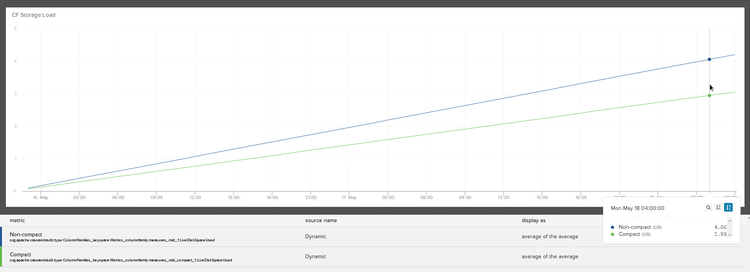
The results showed that, for our use case, the non-compact storage was going to require an overhead of about 35% on storage space (and any additional processing required for that). It was pretty clear that at the data volumes we write at, a 35% tax on storage for non-compact storage was not going to work. So why is there even an option?
One thing to note is that we don’t flatten our data columns into the row. Our data model has always used a blob as the storage object (originally JSON, now ProtoBuf), allowing the application to add/remove columns without modifying the Cassandra schema. If we did expand our columns into the Cassandra schema, the increase would likely be much larger, as each additional column would repeat the column key and timestamp fields.
Why Not Always Use Compact Storage?
Naturally one would wonder why not always use compact storage if it has such a cost savings over non-compact storage. There are a few scenarios where you can’t use compact storage.
Additional Row Columns
As the following shows, you can’t create more than one column past the primary key. Since we saw that compact storage generates a column in the storage model you are limited by the restriction of a single row key, a single column key (built as a multiple-column composite) and a single column data value.
cqlsh:Metrics> CREATE TABLE playlists_3 (   id uuid,   song_id uuid,
           ... title text, artist text,
           ... PRIMARY KEY  (id, song_id )
           ... ) WITH COMPACT STORAGE;
Bad Request: COMPACT STORAGE with composite PRIMARY KEY allows no more than one column not part of the PRIMARY KEY (got: title, artist)
If you require more column values in your data model, you have two options: don’t use compact storage, or serialize them into the single column data value as Json, ProtoBuf, Avro, etc. Updates to columns in that data model will have to be handled application side and must be made atomic within your application. This is important to consider as you won’t be able to leverage Cassandra’s lightweight transactions for updates. For our own use cases we use a mix of Json and ProtoBuf data blobs since our data model is append-only.
Schema Flexibility
Similar to the previous point, a table that is constructed with compact storage cannot be altered after it is created. For example, you can not add or remove columns to a table with compact storage:
cqlsh:Metrics> alter table playlists_1 DROP title;
cqlsh:Metrics> alter table playlists_2 DROP title;
Bad Request: Cannot drop columns from a COMPACT STORAGE table
cqlsh:Metrics> alter table playlists_1 ADD artist text;
cqlsh:Metrics> alter table playlists_2 ADD artist text;
Bad Request: Cannot add new column to a COMPACT STORAGE table
This means you also cannot create indices for additional columns. For example, we couldn’t add an artist column and index the songs by the artist name.
Conclusion
Our primary use case for Cassandra is large time-series data set storage. We must optimize for maximum on-disk efficiency since our storage load and hence costs are directionally proportional to the usage of the service. An extra 35% overhead on the storage footprint is significant.
Time-series data is append-only and is constantly rotating out of the system after some configured TTL. It is often not practical to modify time-series data after it has been written, so any changes to the data format must be done as incremental patches to incoming data. We use descriptive serialization formats like JSON or ProtoBufs to define the data columns allowing us to modify them over time. A schema change can be applied to new data points only, while we continue to support old schema formats until the old data is entirely rotated out.
If storage efficiency isn’t your primary driving factor, then the schema flexibility and transactional updates that a non-compact table provides can make application development easier. Consider how your schema may change over time and whether you want the flexibility to add/remove columns or build additional indices in the future.
Thanks to Mikhail Panchenko of Opsmatic for reviewing an early version of this.
If you enjoyed this article and like working on Cassandra, come work with us!